
Scaling Gauged Inflow Data Using Hydrologic Model Outputs for Better Reservoir Simulations
Published:
Motivation
When building a reservoir simulation model, it is important to validate the model dynamics (e.g., storage and releases) relative to past historical operations. However, these outcomes can be very dependent on the accuracy of the inflow data used to run the simulation.
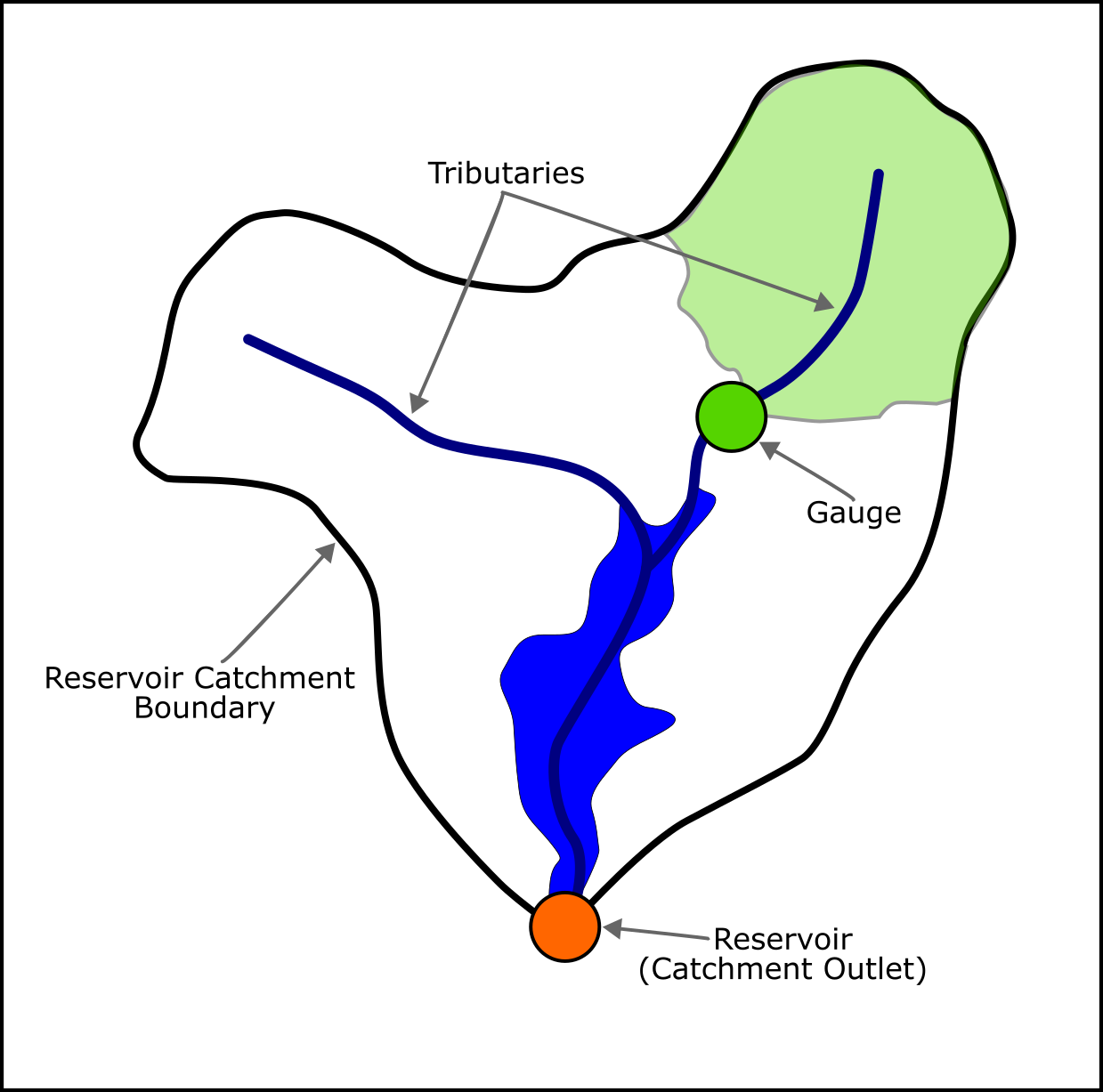
Assuming you have access to gauged reservoir inflow data, it is very likely that the gauge does not capture all of the streamflow into the reservoir since the gauge likely only captures a fraction of the total reservoir catchment.
In Hamilton, Amestoy and Reed (2024), we developed a regression-based inflow scaling technique that uses hydrologic model outputs to estimate time-varying ratios between observed gauge flows and total catchment discharge. When applied in the Delaware River Basin (DRB), the scaled inflows resulted in improved reservoir simulation accuracy compared to using simple observed inflows.
The approach assumes that while hydrologic models may have absolute flow biases, they accurately represent the relative hydrologic processes and scaling relationships between gauged tributaries and total catchment discharge.
Similar inflow-scaling techniques can be found in the literature. For example, Zwart et al. (2023) also used a scaling factor to improve inflow estimates in the DRB. However, these techniques often use a constant scaling coefficient, which ignores the fact that the relative ungauged contributions are dynamic. The method described below accounts for changes in the scaling coefficient across seasons and also for different antecedent hydrologic conditions (high vs low flow conditions).
I am sharing this methodology here since it was found to be valuable in our study (Hamilton et al., 2024) and is broadly applicable in other basins.
If you want more detail about our DRB-specific implementation, I would direct you to:
- the Supporting Information for Hamilton et al. (2024) or
- this Python script which was used to generate the scaled inflow timeseries.
Prerequisite Information
Before we begin, implementation of this scaling method requires, for the catchment of interest:
- Observational gauge flow data from one or more tributaries upstream of the reservoir (green dot in figure)
- Hydrologic model streamflow estimates at the same tributary gauge locations (green dot in figure)
- Hydrologic model streamflow estimates at the catchment outlet (reservoir location; orange dot in figure)
This method is generally compatible with outputs from any hydrologic model which has streamflows at the points described above. In this specific case, I will refer to the National Water Model (NWM) as our hydrologic model of choice as it was used in Hamilton et al. (2024).
Methods
Let $Q_{t}$ represent the unknown total inflow into a reservoir during day $t$. The National Water Model (NWM) provides estimates of total inflow ($Q_{NWM,t}$) as simulated streamflow at the reservoir impoundment location.
The daily scaling coefficient, $c_t$, is defined as the ratio of total reservoir inflow to the sum of $k$-day rolling mean flows at all available upstream gauge stations:
\[c_t = \frac{Q_{t}}{\sum_{i}^{n} \bar{q}_{i,t}}\]where $\bar{q}_{i,t}$ represents the k-day rolling mean flow at gauge station $i$ during day $t$, and $n$ is the number of available gauge stations.
Ordinary Least Squares regression models were used to predict daily scaling coefficients using NWM flows as training data. The assumption is that NWM accurately captures runoff processes and scaling relationships. In our case, the training period spanned 1983-2020 for the NWM dataset.
We developed separate regression models for each meteorological season: winter (December-February), spring (March-May), summer (June-August), and fall (September-November).
The regression model predicts daily scaling coefficients ($\hat{c_t}$) for season $s$ and day $t$:
\[\hat{c_t} = \beta_{0,s} + \beta_{1,s}x_t+\epsilon_t\]where $\beta_{0,s}$ is the seasonal intercept, $\beta_{1,s}$ is the seasonal slope, and the predictor variable $x_t$ is the natural logarithm of summed $k$-day rolling mean observed flows:
\[x_t = \ln\left(\sum^n_i \bar{q}_{i,t}\right)\]The best rolling window length ($k=3$ days) was determined through iterative testing to maximize model R-squared values. It is recommended that you do your own trial and error to test model accuracy for different window sizes.
After the model was trained, we used the observed gauge flows values to calculate the rolling mean value ($x_t$) which was used to predict $\hat{c_t}$.
We made an assumption on the physical constraints, to assume that the scaling coefficient was always equal-to or greater-than 1.0. This may not always be true (e.g., if you are working in a very arid and dry basin) but was appropriate for our context.
After predicting the scaling coefficient, the total inflow was estimated simply as:
\[\hat{Q}_t = \hat{c_t}\sum_{i}^{n} q_{i,t}\]where $q_{i,t}$ represents observed daily flow at gauge station $i$.
Conclusions
If you’ve made it this far, thanks for reading! If you have worked in many reservoir operations contexts you are likely familiar with the inflow data challenges that motivated this method.
Ultimately we developed this method as a relatively simple approach to improve inflow (and consequently model accuracy), and despite it’s simple approach, it worked well for us.
If you have used alternative method to scale inflow data, I’d be curious to hear about them in the comments.
Take care!
References
Hamilton, A. L., Amestoy, T. J., & Reed, P. M. (2024). Pywr-DRB: An open-source Python model for water availability and drought risk assessment in the Delaware River Basin. Environmental Modelling & Software, 181, 106185.
Zwart, J. A., Oliver, S. K., Watkins, W. D., Sadler, J. M., Appling, A. P., Corson‐Dosch, H. R., … & Read, J. S. (2023). Near‐term forecasts of stream temperature using deep learning and data assimilation in support of management decisions. JAWRA Journal of the American Water Resources Association, 59(2), 317-337.