Bayesian Additive Regression Trees for Probabilistic Scenario Discovery

In this post, I provide an argument for using Bayesian Additive Regression Trees (BART) in scenario discovery contexts, highlighting the strengths of the BART model compared to other models used in the literature. I give a very quick introduction to the BART model formulation. Finally, I demonstrate the benefit of using BART for scenario discovery (AKA factor mapping) compared to deterministic Gradient Boosted Tree methods using the Shallow Lake Problem.

In this post I do not provide a comprehensive overview of the theoretical or technical details - for more information about those I’d refer you to the Chipman et al. (2010) publication.

I’ll actually start by jumping to the chase and say that the key strengths of BART are:

• Probabilistic predictions
• Ability to capture non-linear relationships

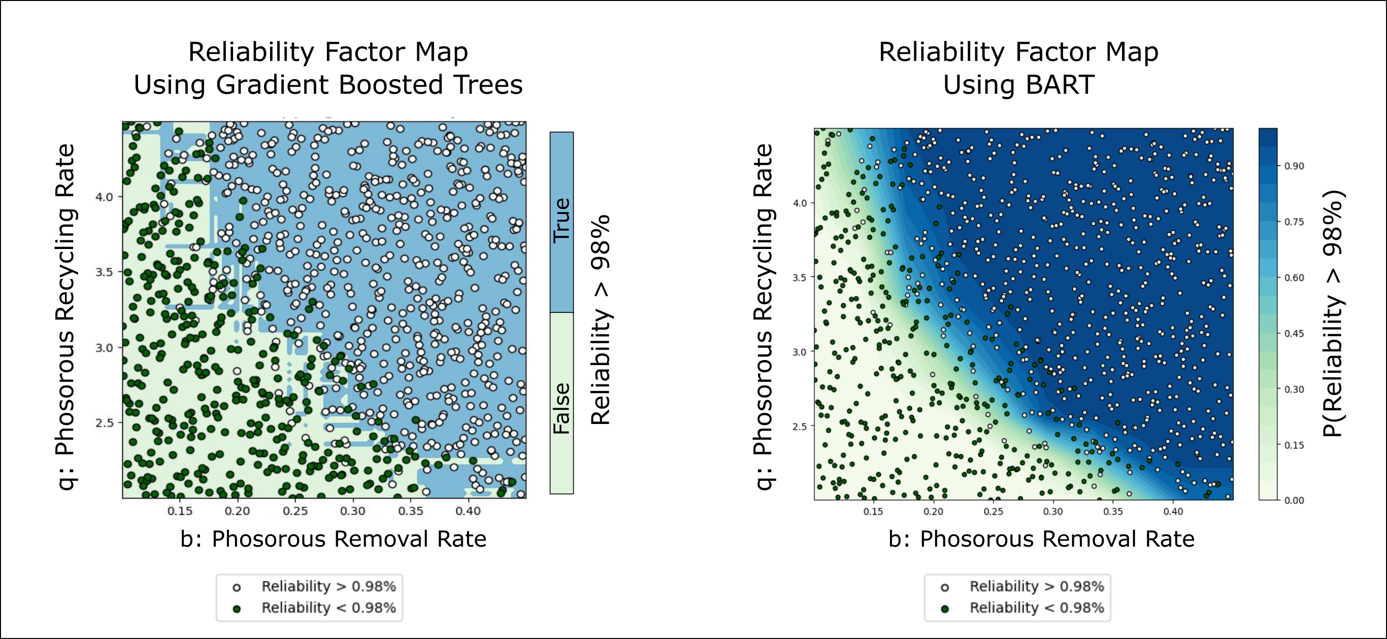
None of the other classification and/or regression models used in the literature can do both of these things simultaneously. In the figure below I show I direct comparison of two scenario discovery results, with one generated using a Gradient Boosted Tree (GBT) model and the other generated using the BART model.

Both models do a good job of capturing the non-linear boundary between the “high reliability” and “low reliability” regions. However, the GBT model inaccurately models this as a deterministic boundary, which it is not. On the other hand, the BART model has the benefit of showing the probabilistic uncertainty around this performance threshold.

Keep reading for more detail!

Review of scenario discovery and commonly used models

Exploratory modeling is a crucial approach in decision-making under deep uncertainty, allowing analysts to investigate complex system behaviors across a wide range of potential futures. A common approach for processing and understanding the performance under uncertainty is scenario discovery, which aim to identify and characterize the key drivers of system performance or failure. These methods help decision-makers understand which combinations of uncertain factors lead to specific outcomes of interest, thereby informing robust policy design.

The most common scenario discovery algorithms I’ve seen used in the exploratory modeling literature are:

• The Patient Rule Induction Method (PRIM)
• Logistic Regression
• Gradient Boosted Trees (GBT)

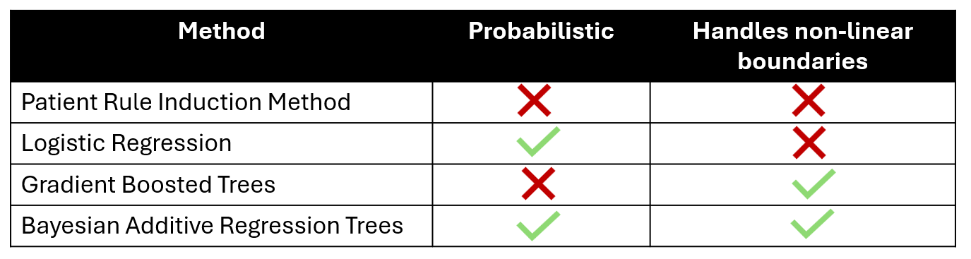
Each of these methods have their own strengths and weaknesses. These weaknesses specifically pertain to the methods ability to (A) handle non-linear boundaries and/or (B) make probabilistic inference.

PRIM is deterministic and unable to capture non-linear boundaries. The logistic regression model has the benefit of including probabilistic predictions, but is limited to linear classification or regression problems. The gradient boosted trees (GBTs) are very strong when it comes to modeling highly nonlinear boundaries, but this is also a deterministic model (no probabilities).

The Bayesian Additive Regression Tree (BART) model, on the other hand, stands out as both having probabilistic inference and being able to handle highly non-linear boundaries.

In our groups most recent work, GBTs have been use because of the ability to model highly non-linear boundaries that manifest in the deeply uncertain exploratory modeling work. These were first used by Bernardo Trindade et al. (2020) when exploring the performance of water management portfolios under uncertainty using WaterPaths. You can see the GBTs used more recently in a recent paper from Lau, Reed, & Gold (2023) in a similar exploratory modeling context that focused on identifying “safe operating spaces” under uncertainty.

Dave Gold wrote a great blog post which gives guidance on the use of GBTs here: “A step-by-step tutorial for scenario discovery with gradient boosted tree”

I view the benefits of GBT methods as being:

• Easy of use. Current packages make it super easy to build, train, and make inferences using the GBT model.
• Ability to assess feature importance.

However, if you look in the literature you may notice that the uncertainty space is not perfectly separable without overfitting the model.

Meaning that there are regions of the uncertainty space where you find “successful” outcomes intertwined with “unsuccessful” outcomes. In these contexts it can be valuable to calculate probabilities of success or failure rather than treating the outcome as a binary classification problem.

For these reasons, I compare the BART model to the GBT model in this post.

A quick introduction to the BART model

This model was first published by Chipman, George and McCulloch (2010) accessed here.

BART is fundamentally an ensemble tree model, similar to Random Forests or Gradient Boosted Trees. In the case of BART, the final prediction is the sum of regression trees, which seek to model the relationship between predictors and a response variable. A key feature of BART is its use of shallow (or weak) prediction trees, typically with only a few terminal nodes, which helps mitigate overfitting.

Because the BART model is built using a Bayesian framework, Markov Chain Monte Carlo (MCMC) methods are required for generating samples of model parameters. MCMC methods are beyond the scope of this post. The key here is that the result of the MCMC sampling process is a set of samples describing the posterior distribution of BART model parameters, conditional on the training data.

In other words, the MCMC produces a large number of different tree parameters (splits and terminal node prediction values) which represent the posterior distribution of parameters. We can then use this set of parameter values to produce a posterior distribution of the final prediction.

Using the notation:

• $T$ is a binary tree consisting of a set of decision rules and terminal nodes
• $M = {\mu_1, \mu_2, \dots, \mu_b}$ is the set of parameter values with each $b$ terminal node of $T$
• $g(x; T,M)$ is a step function that assigns $\mu_i \in M$ to a certain value $x$ and represents the regularization from the BART prior
• $Y$ a prediction

A single tree takes the form:

A sum of trees is then:

The BART model has 3 primary hyperparameters: the number of trees (m), and two regularization parameters (alpha, beta). The two regularization priors are used to limit the depth of the prediction trees.

The regularization priors define the probability of a node splitting at depth (d), using the funciton:

In Chapman et al. (2010), they recommend $\alpha=0.95$ and $\beta=2$, which results in the high probabilities for small trees.

Demo: BART for Scenario Discovery in the Shallow Lake Problem

Given that the Shallow Lake Problem shows up frequently in this post, I am going to exclude the fine details of the context, model, and problem formulation. If you’d like to study the Lake Problem in more depth, I’d recommend you read the publication from Quinn et al. (2017), view the Lake Problem Training series on our Lab Manual site or search around for other posts on the blog.

The shallow lake problem is used as a theoretical environmental management problem that illustrates the difficultly of finding management policies that balance multiple different objectives while avoiding irreversible ecological tipping points.

In this problem, a managers must balance the Town’s agricultural and industrial productivity with the pollution it creates in a downstream lake. Too much phosphorous pollution will cause irreversible eutrophication of the lake.

The model of phosphorous in the lake ($X_t$) at time t is governed by:

Where:

• $a_t$ is the town’s pollution release at each timestep
• $b$ is the natural decay rate of phosphorous in the lake
• $q$ defines the lake’s natural phosphorous recycling rate, when phosphorous is moved from the sediment back into the water column
• $\varepsilon$ represents uncontrollable natural inflows of pollution modeled as a log-normal distribution with a given mean, $\mu$, and standard deviation, $\sigma$.

Importantly, many of the parameters that are used to describe the natural processes (b, q, mu, sigma) are deeply uncertain but have a big impact on whether or not the lake tips into the eutrophic state.

The Town’s main objective is to maximize reliability, expressed as the likelihood of avoiding eutrophication over the planning horizon. The managers want to make sure the final policy has a reliability of at least 98%, to increase the confidence that they will avoid eutrophication.

Let’s assume that the managers have identified a policy, and want to measure the reliability of this policy under a range of differently deeply uncertain conditions relating to the ecological parameters.

In this case, we simulate the policy for many different uncertainty states, and then use scenario discovery to identify the ecological conditions that lead to eutrophication.

In this case, I’ve loaded some existing samples of the uncertain factors (or “states or the world”) from prior study by Quinn et al. (2017).

These inputs include difference combinations of uncertain ecological factors, which are then used to evaluate the policy performance using a simulation model of the lake dynamics. I also load the reliability data which corresponds to simulation model outputs.

Reliability is calculated as the fraction of the time that the lake is not in the eutrophic state, based on the simulation results.

The inputs.txt and reliability.txt files were shared with the original post on WaterProgramming, in case you would like to download and follow along:

import numpy as np
import pandas as pd
from sklearn.preprocessing import StandardScaler
import matplotlib.pyplot as plt

# load inputs.txt and reliability.txt
inputs = pd.read_csv('inputs.txt', header=None, sep=' ')
inputs.columns = ['b', 'q', 'mu', 'sigma', 'delta']
inputs = inputs.drop(columns=['delta'])
inputs = inputs.values

# Reliability values = % of samples that avoid eutrophication
reliability = pd.read_csv('reliability.txt', header=None)
reliability = reliability.values.flatten()/100

Now comes the definition of the BART model.

Here, I use the PyMC-BART package to construct and use the inference model. In my prior post “Introduction to Bayesian Regression using PyMC” I gave a bit of commentary on how to formulate a PyMC model. The PyMC-BART variant follows a similar model formulation.

A few things to consider are:

• The number of trees (n_trees) controls the model complexity. More trees will enable more complex dynamics to be modeled, but will require more computation time during the MCMC sampling.
• The number of MCMC samples to generate (n_samples). Use a larger number of samples is necessary for model complex posterior distributions.
• Use of a TruncatedNormal distribution. I want to constrain my model outputs at 0.0 and 1.0, since those are the bounds on my reliability metric.

import pymc as pm
import pymc_bart as pmb

# Number of trees to include in BART model
n_trees = 30

# Number of MCMC samples to draw
n_samples = 1000

# Defining the model
with pm.Model() as model:
    X = pm.Data('X', inputs)
    n_points = X.shape[0]

    w = pmb.BART("w", X=X, 
                 Y=reliability, 
                 m=n_trees,
                 shape=(n_points))
    
    y_sigma = pm.HalfCauchy('y_sigma', beta=0.5, shape=(1))
    y_pred = pm.TruncatedNormal("y", 
                      mu=w, sigma=y_sigma,
                      lower=0.0, upper=1.0,  
                      observed=reliability, 
                      shape=(n_points))
    
    # MCMC sampling
    trace = pm.sample(n_samples, tune=500, cores=4, target_accept=0.9)

When using the pm.sample() function, we initiate the MCMC algorithm which is going to repeatedly sample, test, and update the set of values defining the posterior distribution of BART parameters. This can be pretty computationally intensive and may take 3-5 minutes depending on your setup.

Once the MCMC sampling is complete, the trace variable will contain all of the posterior distribution samples, defining the empirical posterior distribution for each set of environmental uncertainties.

After running the MCMC sampling scheme, I want to then make posterior predictions across a grid of factor values, so that I can have continuous reliability estimates across the entire uncertainty space (not just at my initial SOW values). This is commonly done in other GBT methods as well.

To do this, I need to first create a grid of uncertain factor values, then re-organize the grid values into a $[N, 4]$ matrix that matches my BART model input dimensions.

# Meshgrid to factor values 
# used to generate posterior predictions
x_test_pts = []
for i in range(inputs.shape[1]):
    x_test_pts.append(np.linspace(inputs[:, i].min(), inputs[:, i].max(), 10))
x_grid = np.meshgrid(*x_test_pts)

# Reformat to match BART input dims
x_test = np.c_[[grid.ravel() for grid in x_grid]].T

With my grid of new uncertain factor values, I am going to generate posterior distributions of reliability at each point in x_test using the PyMC pm.sample_posterior_predictive() function:

with model:
    # set the new values as the X varaible
    pm.set_data({'X':x_test})
    
    # generate posterior samples
    posterior = pm.sample_posterior_predictive(trace, predictions=True)

# reformat into shape [4000, 1] by flattening MCMC draws from different chains
y_pred = posterior.predictions['y'].data
y_pred = y_pred.reshape((y_pred.shape[0]*y_pred.shape[1], y_pred.shape[2]))

Now I have a multi-dimensional posterior dataset that includes 4,000 posterior samples of reliability estimates at each grid point in my uncertainty space.

Rather than trying to plot this multi-dimensional distributional data, I want to do one final transformation to determine the empirical probability that Reliability is greater than the target 98% based on the posterior samples.

# calculate the probability that reliability > 98% based on posterior samples
prob_success = (y_pred > 0.98).sum(axis=0)/y_pred.shape[0]

# reshape to match the grid dimenisons for plotting
z = prob_success.reshape(x_grid[0].shape)

Finally I am ready to produce the contour plot, showing the probability that reliability is greater than 98% for any combination of uncertain ecological factors:

# plotting contour factor map
plt.figure(figsize=(10,7))

plt.contourf(x_grid[0][:,:,0,0], x_grid[1][:,:,0,0], z[:,:,0,0], levels=20,cmap='GnBu',
             vmin=0.0, vmax=1.0)
plt.colorbar()

# Add original SOW points as binary success based on satsifying reliability condition
success = reliability > 0.98
plt.scatter(inputs_original.loc[success==True, 'b'], 
            inputs_original.loc[success==True, 'q'], 
            c='white', 
            cmap='bwr_r',s=20, edgecolor='k', 
            label='Reliability > 0.98%')
plt.scatter(inputs_original.loc[success==False, 'b'], 
            inputs_original.loc[success==False, 'q'], 
            c='darkgreen', 
            cmap='bwr_r',s=20, edgecolor='k', 
            label='Reliability < 0.98%')
plt.legend(loc='upper center', bbox_to_anchor=(0.5, -0.1))
plt.show()

In the figure below, I show the output of this BART scenario discovery (on the right) compared to a similar result generated by the GBT method.

Of course, both models do a sufficient job and identifying the non-linear tipping point boundary (boundary between low and high reliability) but the BART model is able to reflect the non-deterministic nature of this boundary.

References

• Hugh A. Chipman. Edward I. George. Robert E. McCulloch. “BART: Bayesian additive regression trees.” Ann. Appl. Stat. 4 (1) 266 - 298, March 2010. https://doi.org/10.1214/09-AOAS285
• Quinn, J. D., Reed, P. M., & Keller, K. (2017). Direct policy search for robust multi-objective management of deeply uncertain socio-ecological tipping points. Environmental Modelling & Software, 92, 125-141.
• Trindade, B. C., Gold, D. F., Reed, P. M., Zeff, H. B., & Characklis, G. W. (2020). Water pathways: An open source stochastic simulation system for integrated water supply portfolio management and infrastructure investment planning. Environmental Modelling & Software, 132, 104772.
• Lau, L. B., Reed, P. M., & Gold, D. F. (2023). Evaluating Implementation Uncertainties and Defining Safe Operating Spaces for Deeply Uncertain Cooperative Multi‐City Water Supply Investment Pathways. Water Resources Research, (7), e2023WR034841.