
An Introduction to Linear Programming for Reservoir Operations (Part 1)
Published:
Originally published on the WaterProgramming blog. The formulation below reflects the revised version of the post, which optimizes both releases and storage over multiple timesteps. See Part 2 for the Python implementation using Pyomo.
Motivation:
If you are like me, you may have a baseline knowledge of linear programming (LP) methods, but may not have worked with the topic in a hands-on way, as opposed to the abstract/generic formulation that is often presented in lectures. This post is for the hydrology enthusiasts out there who want to experiment with linear programming methods in a way that makes sense to them.
In this post, I provide a very brief intro to linear programming then go through the process of applying a linear programming approach to a simple hydroelectric reservoir problem focused on determining a release rate that will consider both storage targets and energy generation. In a later post, I will come back to show how the formulation generated here can be implemented within simulation code.
Content:
- An introduction to linear programming
- Formulating an LP
- Solving LP problems: Simplex
- Relevance for water resource managers
- A toy reservoir demonstration
- The problem formulation
- Constraints
- Objective
- The problem formulation
- Conclusions and what’s next
An introduction to linear programming
Linear programming (LP) is a mathematical optimization technique for making decisions under constraints. The aim of an LP problem is to find the best outcome (either maximizing or minimizing) given a set of linear constraints and a linear objective function.
Formulating an LP
The quality of an LP solution is only as good as the formulation used to generate it.
An LP formulation consists of three main components:
1. Decision Variables: These are the variables that you have control over. The goal here is to find the specific decision variable values that produce optimal outcomes. There are two decision variables shown in the figure below, x1 and x2.
2. Constraints: These are the restrictions which limit what decisions are allowed. (For our reservoir problem, we will use constraints to make sure total mass is conserved, storage levels stay within limits, etc.) The constraints functions are required to be linear, and are expressed as inequality relationships.
3. Objective Function: This is the (single) metric used to measure outcome performance. This function is required to be linear and it’s value is denoted Z in the figure below, where it depends on two decision variables (x1, and x2).
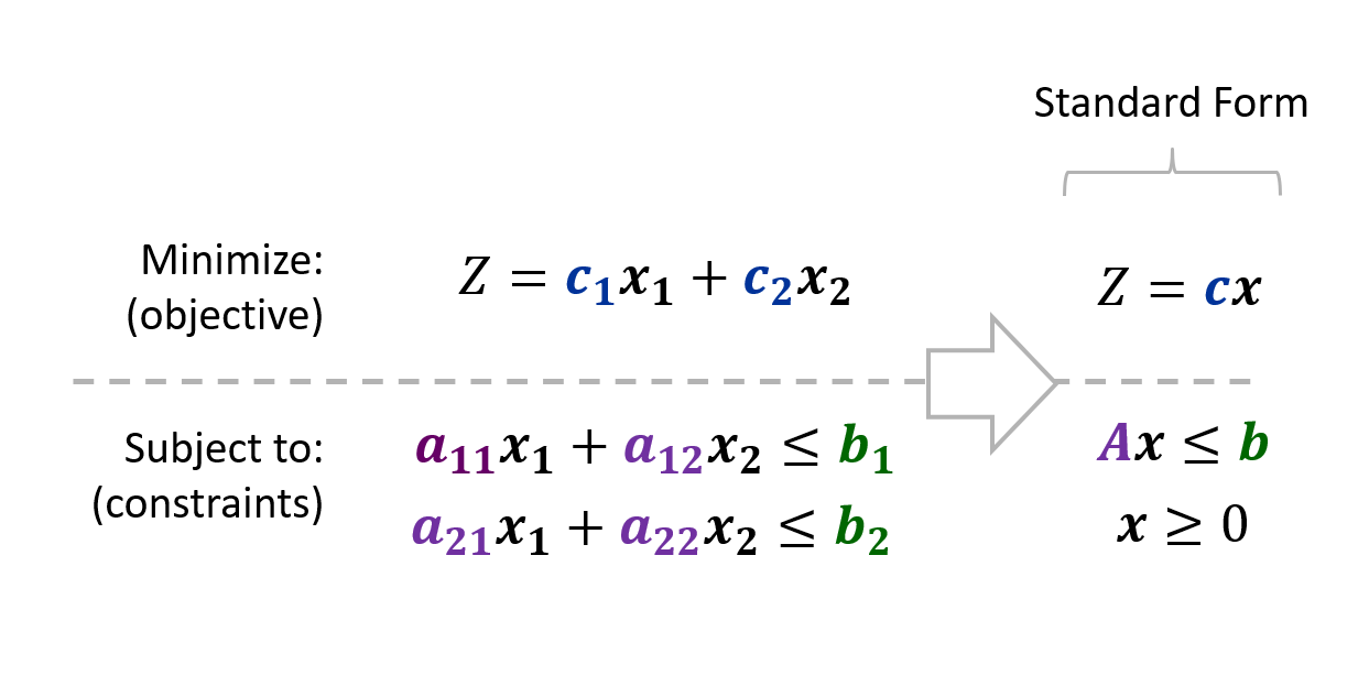
In practice, the list of constraints on the system can get very large. Fortunately matrix operations can be used to solve these problems quickly, although this requires that the problem is formatted in “standard form” shown above. The standard form arranges the coefficient values for the constraints within matrices A and b.
Solving LP problems: keep it Simplex
Often the number of potential solutions that satisfy your constraints will be very large (infinitely large for continuous variables), and you will want to find the one solution in this region that maximizes/minimizes your objective of interest (the “optimal solution”).
The set of all potential solutions is referred to as the “feasible space” (see the graphic below), with the constraint functions forming the boundary edges of this region. Note that by changing the constraints, you are inherently changing the feasible space and thus are changing the set of solutions that you are or are not considering when solving the problem.
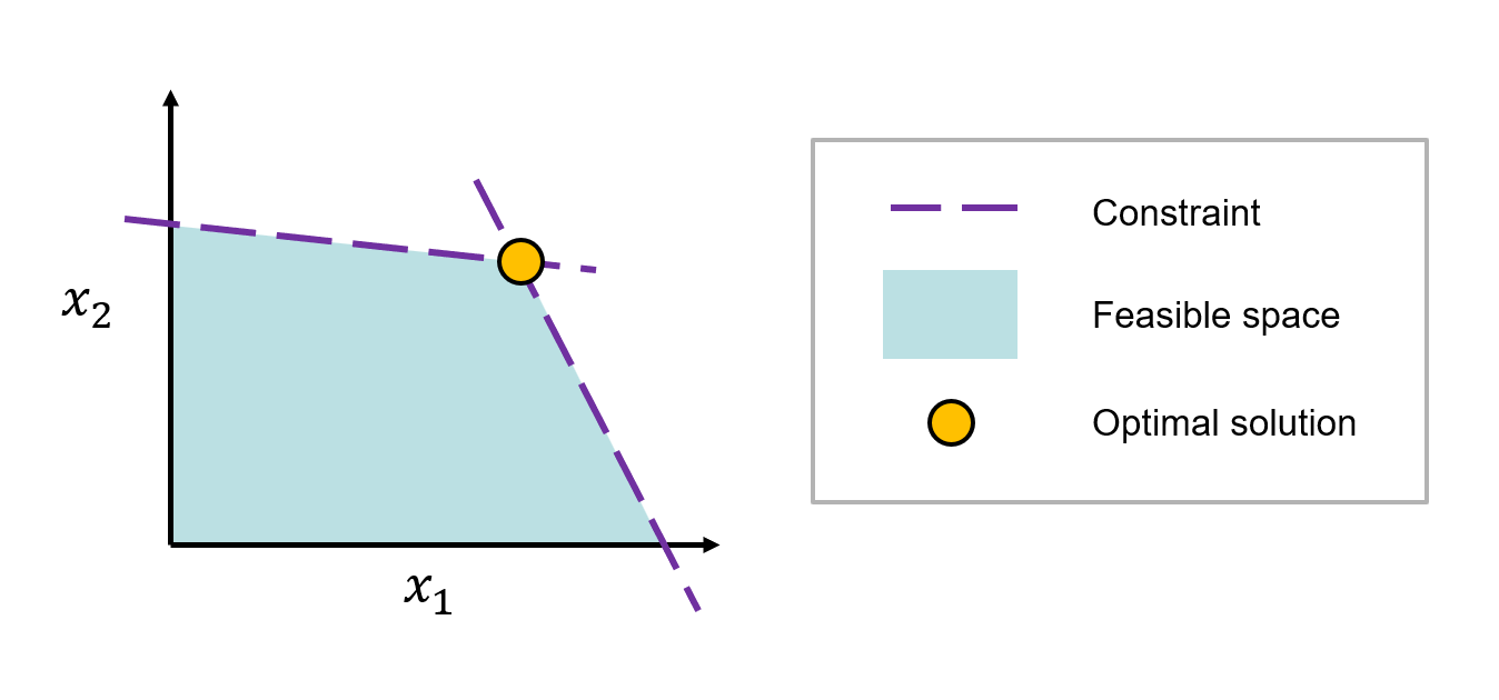
The fundamental theorem of linear programming states that the optimal solution for an LP problem will exist at one of corners (or a vertex) of the feasible space.
Recognizing this, George Dantzig proposed the Simplex algorithm which strategically moves between vertices on the boundary feasible region, testing for optimality until the best solution is identified.
A detailed review of the Simplex algorithm warrants it’s own blog post, and wont be explained here. Fortunately there are various open LP solvers. For example, one option in Python is scipy.optimize.linprog().
Relevance for water resource managers
Why should you keep read this post?
If you work in water resource systems, you will likely need to make decisions in highly constrained settings. In these cases, LP methods can be helpful. In fact there are many scenarios in water resource management in which LP methods can (and historically have) been useful. Some general application contexts include:
- Resource allocation problems: LP can be used to allocate water efficiently among different users like agriculture, industry, and municipalities.
- Operations optimization: LP can guide the operations decisions of water reservoirs, deciding on storage levels, releases, and energy production to maximize objectives like water availability or energy generation from hydropower (the topic of this demonstration below).
Toy Reservoir Demonstration: Problem Formulation
The following demo aims to provide a concrete example of applying linear programming (LP) in the realm of water resource management. We will focus on a very simple reservoir problem, which, despite its simplicity, captures the essence of many real-world challenges.
Imagine you are managing a small hydroelectric reservoir that provides water and energy to a nearby town. Your goal is to operate the reservoir, choosing how much water to release each day such that the (1) the water level stays near a specific target and (2) you maximize energy generation. Additionally, there is a legally mandated minimum flow requirement downstream to sustain local ecosystems
Here, I will translate this problem context into formal LP notation, then in a later post I will provide Python code to implement the LP decision making process within a simulation model.
Problem formulation
We want to translate our problem context into formal mathematical notation that will allow us to use an LP solver. In order to help us get there, I’ve outlines the following table with all the variables being considered here.
| Term | Description |
|---|---|
| $I_t$ | Inflow into the reservoir at time $t$ |
| $D_t$ | Consumptive water demand at time $t$ |
| $S_t$ | Storage in the reservoir at time $t$ |
| $R_t$ | Reservoir release decision during time $t$ |
| $R_{min}$ | The minimum required reservoir release |
| $R_{max}$ | The maximum possible reservoir release |
| $E_t$ | Energy produced during time $t$ |
| $\eta$ | Energy conversion coefficient |
Decision variables
In this case the things we are controlling at the reservoir releases (Rt), and the storage level (St) at each timestep.
Constraints:
Constraints are the backbone of any LP problem, defining the feasible space which ultimately dictates the optimal solution. Without constraints, an LP problem would have infinite solutions, rendering it practically meaningless. Constraints are meant to represent any sort of physical limitations, legal requirements, or specific conditions that must be satisfied by your decision. In the context of water resource management, constraints could signify capacity limits of a reservoir, minimum environmental flow requirements, or regulatory water diversion limits.
- Mass balance requirement: Naturally you want to make sure that mass is conserved through the reservoir, by balancing all of the inflows, outflows and storage states, for each timestep (t):
Although we need to separate this into two separate inequalities in order to meet the “standard form” for an LP formulation. I am also going to move the decision variables (Rt and St) to the left side of the inequalities.
\[S_{t}-S_{t-1} +R_{t}\leq I_{t} - D_{t}\] \[-S_{t}+ S_{t-1} -R_{t}\leq -(I_{t} - D_{t})\]- Storage limitations:
The most obvious constraints are that we don’t want the reservoir to overflow or runout of water. We do this by requiring the storage to be between some minimum (Smin) and maximum (Smax) values specified by the operator.
Again we need to separate this into two separate inequalities:
\[S_{t} \leq S_{max}\] \[-S_{t}\leq -S_{min}\]- Maximum and minimum release limitations: The last two constraints represent the physical limit of how much water can be discharged out of the reservoir at any given time (Rmax) and the minimum release requirement that is needed to maintain ecosystem quality downstream of the reservoir (Rmin).
Objective:
The objective function in an LP represents your goals. In the case of our toy reservoir, we have two goals:
- Maximize water storage
- Maximize energy production.
Initially when I was setting this demonstration up, there was no hydroelectric component. However, I chose to add the energy generation because it introduces more complexity in the actions (as we will see). This is because the two objectives conflict with one another. When generating energy, the LP is encouraged to release a lot of water and maximize energy generation, however it must balance this with the goal of raising the storage to the target level. This tension between the two objectives makes for much more interesting decision dynamics.
- Objective #1: Maximize storage Since our reservoir managers want to make sure the Town’s water supply is reliable, they want to maximize the storage. This demo scenario assumes that flood is not a concern for this reservoir. We can define objective one simply as:
- Objective #2: Maximize energy generation: Here I introduce a second component of the objective function associated with the amount of hydroelectric energy being generated by releases. Whereas the minimize-storage-deviation component of the objective function will encourage minimizing releases, the energy generation component of the objective function will incentivize maximizing releases to generate as much energy each day as possible.
Under these conditions, I will define the energy generated as:
\[O_2 = \eta R_{t}\]- Aggregate minimization objective: Lastly, LP problems are only able to solve for a single objective function. With that said, we need to aggregate the storage and energy generation objectives described above. In this case I take a simple sum of the two different objective scores. Of course this is not always appropriate, and the weighting should reflect the priorities of the decision makers and stakeholders.
In this case, this requires a priori specification of objective preferences, which will determine the solution to the optimization. In later posts I plan on showing an alternative method which allows for posterior interpretation of objective tradeoffs. But for now, we stay limited with the basic LP.
Also, we want to formulate the optimization as a minimization problem. Since we are trying to maximize both of our objectives, we will make them negative in the final objective function.
The final aggregate objective is:
\[Z = -\sum^N_{t=0} (O_{1,t} + O_{2,t})\] \[Z = -\sum^N_{t=0} (\eta R_{t}+S_{t})\]Final formulation:
As we prepare to solve the LP problem, it is best to lay out the complete formulation in a way that will easily allow us to transform the information into the form needed for the solver:
Minimize: $Z = -\sum^N_{t=0} (\eta R_{t}+S_{t})$
Such that $\forall{t}$:
\[\begin{align} S_{t}-S_{t-1} +R_{t}\leq I_{t} - D_{t}\\ -S_{t}+S_{t-1} -R_{t}\leq -(I_{t} - D_{t})\\ S_{t} \leq S_{max} \\ -S_{t}\leq -S_{min} \\ R_{t} \leq R_{max}\\ -R_{t} \leq - R_{min}\\ \end{align}\]Caveats, conclusions, and what’s next
If you’ve made it this far, good on you, and I hope you found some benefit to the process of formulating a reservoir LP problem from scratch.
This post was meant to include simulated reservoir dynamics which implement the LP solutions in simulation. However, the post has grown quite long at this point and so I will save the code for another post. In the meantime, you may find it helpful to try to code the reservoir simulator yourself and try to identify some weaknesses with the proposed operational LP formulation.
To add some brief caveats, this model is very simple and not suitable for practical implementation. This is largely due to the single-day foresight. In practice, you would want to include a longer time-horizon during the optimization such that you can solve for a timeseries of releases/storages that seek to optimize the performance over the full time horizon. We will see this weakness manifest in the in the implementation and I may later expand the demo to include longer time horizons.
Thanks for reading, and see you here next time where we will use this formulation to implement release decisions in a reservoir simulation.