An Introduction to Linear Programming for Reservoir Operations (Part 2): Implementation with Pyomo

Introduction

Previously, in Part 1 I used a very simple reservoir operations scenario to demonstrate some linear programming (LP) concepts.

After some feedback on my initial formulation I went back and revised the formulation to make sure that (1) both reservoir releases and storage levels are optimized simultaneously and (2) the LP handles decisions over multiple timesteps (1,…,N) during optimization. Definitely look back at Part 1 for more context.

The current LP formulation is as follows:

Minimize Z (which maximizes energy production and storage level):

Such that for each timestep, $\forall{t}$ :

In this post, I show a simple implementation of this LP using the Pyomo package for solving optimization problems in Python.

I have shared the code used in this demo in a repository here: TrevorJA/Reservoir-LP-Demo

Constructing the LP model with Pyomo

While Pyomo can help us construct the LP model, you will need access to a separate solver software in order to actually run the optimization. I don’t get into the details here on how to set up these solvers (see their specific installation instructions), but generally you will need this solver to be accessible on you PATH.

Two solvers that I have had good experience with are:

• SCIP Optimization Suite (used here)
• GNU Linear Programming Kit

As always, it’s best to consult the Pyomo documentation for any questions you might have. Here, I highlight a few things that are needed for our implementation.

We start by importing the pyomo.environ module:

import pyomo.environ as pyo

From this module we will need to use the following classes to help build our model:

• pyo.ConcreteModel()
• pyo.RangeSet()
• pyo.Var()
• pyo.Objective()
• pyo.Constraint()
• pyo.SolverFactory()

The nice thing about using pyomo rather than trying to manage the LP matrices yourself is that you can specify objectives and constraints as functions.

For example, the objective function is defined as:

# Objective Function
def objective_rule(m):
    return -sum((eta_0 * m.R[t]) + (m.S[t]/S_max*100) for t in m.T)

And a constraint used to enforce the lower limit of the storage mass balance can defined as:

def S_balance_lower(m, t):
    if t == 0:
        return m.S[t] + m.R[t] <= initial_storage + I[t] - D[t]
    return m.S[t] + m.R[t] <= m.S[t-1] + I[t] - D[t]

Rather than picking the full implementation apart, I present the entire function below, and encourage you to compare the code implementation with the problem definition above.

def pyomo_lp_reservoir(N, S_min, S_max, R_min, R_max, 
                       eta_0, I, D,  
                       initial_storage,
                       R_change_limit=None):

    # Model
    model = pyo.ConcreteModel()

    # Time range
    model.T = pyo.RangeSet(0, N-1)  

    # Decision Variables
    model.S = pyo.Var(model.T, bounds=(S_min, S_max))  # Storage
    model.R = pyo.Var(model.T, bounds=(R_min, R_max))  # Release

    # Objective Function
    def objective_rule(m):
        return -sum((eta_0 * m.R[t]) + (m.S[t]/S_max*100) for t in m.T)
    model.objective = pyo.Objective(rule=objective_rule, sense=pyo.minimize)

    # Constraints
    def S_balance_lower(m, t):
        if t == 0:
            return m.S[t] + m.R[t] <= initial_storage + I[t] - D[t]
        return m.S[t] + m.R[t] <= m.S[t-1] + I[t] - D[t]

    def S_balance_upper(m, t):
        if t == 0:
            return -(m.S[t] + m.R[t]) <= -(initial_storage + I[t] - D[t])
        return -(m.S[t] + m.R[t]) <= -(m.S[t-1] + I[t] - D[t])
    model.S_lower = pyo.Constraint(model.T, rule=S_balance_lower)
    model.S_upper = pyo.Constraint(model.T, rule=S_balance_upper)
    model.S_final = pyo.Constraint(expr=model.S[N-1] == initial_storage)
    
    # Solve
    solver = pyo.SolverFactory('scip')
    results = solver.solve(model)

    if results.solver.status == pyo.SolverStatus.ok:
        S_opt = np.array([pyo.value(model.S[t]) for t in model.T])
        R_opt = np.array([pyo.value(model.R[t]) for t in model.T])
        return S_opt, R_opt
    else:        
        raise ValueError('Solver did not converge')

Note that in this implementation, pyomo will optimize all of the reservoir release and storage decisions simultaneously, returning the vectors of length N which prescribe the next N days of operations.

Note the assumption of perfect foresight: In order to use this LP approach, we need to have information concerning the reservoir inflow and demand for the next N days. In this simple demo, it is assumed that the operators have perfect forecasts of these values into the future. Of course this is not practical, but for the purpose of this demo we will not introduce any more advanced approaches.

Usage

Now we are ready to use our LP reservoir simulator. In the code block below, I set some specifications for our operational constraints, generate fake inflow and demand timeseries, run the LP solver, and plot the simulated results:

# spcifications
N_t = 30
S_min = 2500
S_max = 5000
R_min = 10
R_max = 1000
eta = 1.2

# Generate simple inflow and demand data
I, D = generate_data(N_t, correlation_factor = -0.70,
                     inflow_mean=500, inflow_std=100,
                     lag_correlation=0.2)


# Run LP operation simulation
S_sim, R_sim = pyomo_lp_reservoir(N_t, S_min, S_max, R_min, R_max, eta, I, D, 
                                  initial_storage=S_max)

# Plot results
plot_simulated_reservoir(I, D,
                         R_sim, S_sim, 
                         S_max, eta=eta)

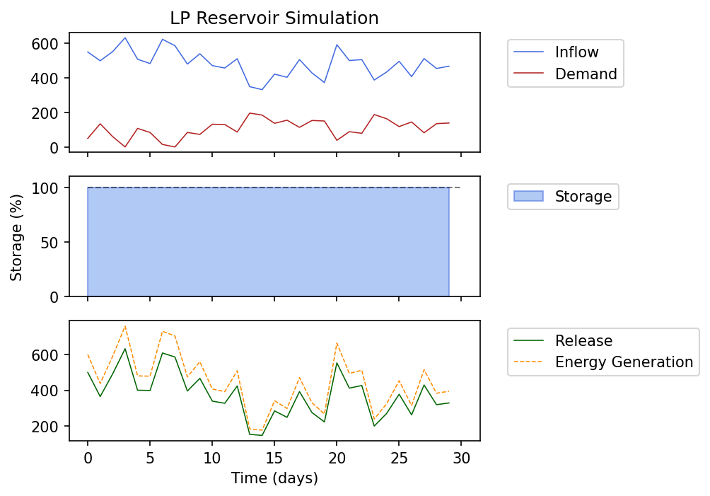
Under this LP formulation, with a perfect inflow forecast, the reservoir operates as a “run of river” with the release rates being very close to the inflow rate.

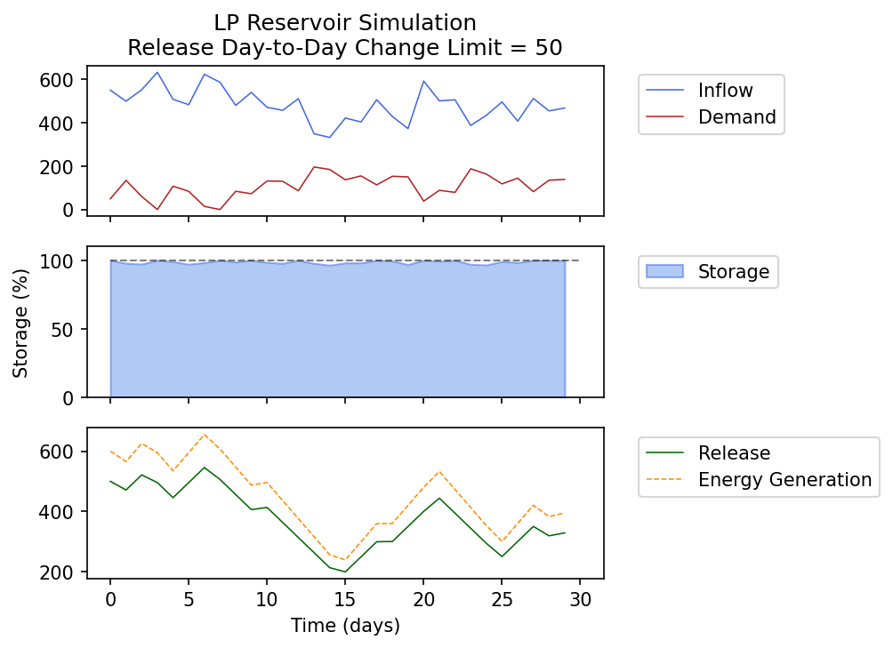
In practice, operators may need to limit the difference in release volume from day-to-day. I added an optional parameter (R_change_limit) which adds a constraint on the difference subsequent releases from between each day.

The operations, with the daily release change rate limited to 50 is shown below.